
How Claude changed how we decide what to bring in, and when
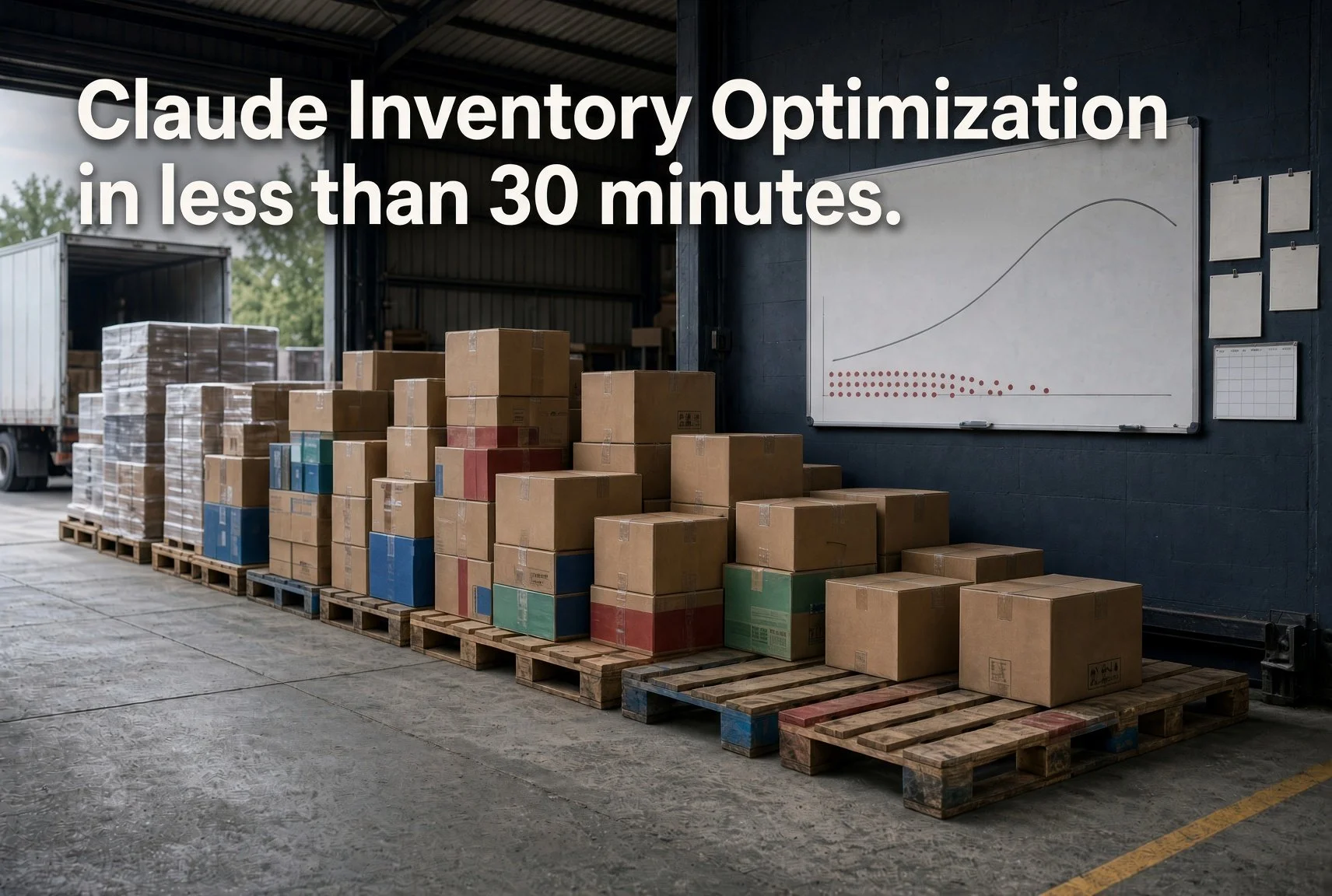
Most inventory teams already have the data. What they lack is a way to turn a messy question into a decision before the next truck is scheduled. In two recent projects, Claude was connected directly to Power BI semantic models, so it worked from the same SKU, order, receipt, and forecast measures the planners already trust. No spreadsheet export. No second version of the truth.
Choosing the right 20 pallets
An acquisition left a company with mixed-SKU pallets in two external warehouses. Internal space limitations dictate that this company can’t call in more than 20 pallets. The goal was not to empty a warehouse. It was to bring in the smallest set of pallets that covers the most urgent needs.
The priorities were explicit. First, cover open orders that internal stock cannot fill. Second, favor older inventory over newer receipts. Third, extend coverage against the forecast so the next few weeks are not spent calling the same warehouses again.
In mathematical terms, this is a cardinality-constrained weighted set-cover problem. Each pallet is a set of SKUs. Each SKU carries a weight based on open-order shortfall, then forecasted demand, with an age bias so older stock scores higher. The solver must choose at most 20 sets to maximize total weighted coverage, without double-counting a SKU that appears on more than one pallet.
Claude read pallet contents, open orders, on-hand, and forecast from the semantic model, scored each pallet, and returned a call-in list with the SKUs each pallet uniquely covers. Planners could see why pallet 14 beat pallet 31, and what demand would still be exposed if they stopped at 15 pallets instead of 20. The constraint did the work. The model did not invent a new policy. It enforced the one the business already had. A prior attempt to code this in Excel bogged down the software rendering Excel ineffective.
Finding out when the stockouts actually happened
The second project started with a belief most teams share: we stock out in peak season because demand spikes. Claude was asked to study a full year of out-of-stocks against the seasonal calendar already defined in the model.
The pattern ran the other way. Most stockouts landed in the off-season. Good news there! Peak was protected. The quiet months were not. That single finding changed the conversation from “we need more safety stock before peak” to “we are letting the pipeline run dry after peak and paying for it later.”
Claude then estimated lost revenue by applying the selling price and the unfilled demand already sitting in the model, so the number was traceable to measures finance already uses. It also compared actual receipt lead times with the supplier lead times stored in the system. Where actual lead time ran longer, it flagged the SKUs that should be ordered earlier for the next peak, with the gap stated in days rather than as a vague “order sooner.”
The useful output was not a dashboard. It was a short list: these items, this many days earlier, this much revenue left on the table last year when the same gap was ignored.
What the connection changed
In both cases the advantage was the semantic model, not a clever prompt. Claude could ask the same measures a planner would, then do the comparison a person cannot do across thousands of SKU-pallet or SKU-week combinations in an afternoon. The business owner still set the constraint (20 pallets) and the priority (orders first, then age, then forecast). The model enforced them and showed the tradeoff.
If your inventory questions sound like “which of these should we bring in” or “when did we actually run out, and what did it cost,” the bottleneck is rarely another report. It is getting an optimizer and an analyst to read the model you already built.