
Optimizing Inventory Management for Seasonal Businesses: Safety Stock and Reorder Point Strategies
In the dynamic world of supply chain and operations, effective inventory management is crucial for maintaining customer satisfaction while minimizing costs. For businesses with seasonal demand fluctuations, such as retailers dealing in holiday goods, agricultural suppliers, academic retail or tourism-related products, traditional inventory methods can fall short.
This article explores the safety stock and reorder point approach, with a focus on adapting it for seasonal variations. I'll delve into the standard year-round calculation and contrast it with a dual-season method, highlighting the pros and cons of each to help operations professionals, like you, make informed decisions.
Understanding Safety Stock and Reorder Point
Before diving into seasonal adaptations, let's recap the basics. Safety stock is the extra inventory held to buffer against uncertainties like demand spikes, supply delays, or forecasting errors. It's calculated using factors such as average daily demand, lead time (the time from ordering to receiving goods), and service level (the desired probability of not stocking out).
The formula for safety stock is typically:
Safety Stock = Z × √(Lead Time) × σ_D
where:
Z is the Z-score corresponding to the service level (e.g., 1.65 for 95% service level),
σ_D is the standard deviation of daily demand.
The reorder point (ROP) determines when to place a new order:
ROP = (Average Daily Demand ×Lead Time) + Safety Stock
These metrics ensure inventory doesn't dip below zero during replenishment periods. In a stable business, one set of calculations suffices. But for seasonal operations, demand isn't constant. Peaks can surge to demand levels that are many multiples of the off-peak volume, demanding a tailored strategy.
The Challenge of Seasonality in Inventory Management
Seasonal businesses face predictable yet volatile demand cycles. For one of my retail clients, the overall volume is quite predictable, but the 4-month peak season coupled with variable lead times from suppliers, minimum order quantities and a desire for shipping efficiencies make it challenging to get both the timing and the quantities just right.
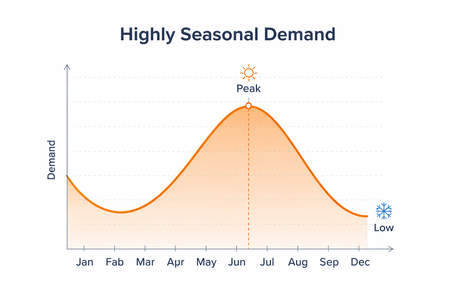
Imagine a company selling winter apparel: sales skyrocket from November to February (peak season) but plummet in the warmer months (off-peak). Using a single, averaged calculation for the entire year ignores these swings, leading to inefficiencies. This often results in excess inventory during the off-peak period, tying up capital and increasing holding costs like storage, insurance, and obsolescence risks.
To address this, many businesses adopt a segmented approach: calculating separate safety stock and ROP values for peak (e.g., 4 months) and off-peak (e.g., 8 months) periods. This requires historical data segmented by season, accurate forecasting tools (like time-series analysis), and periodic reviews to switch between the two sets.
Implementing the Dual-Season Method
Data Segmentation: Divide your historical sales data into peak and off-peak periods. For peak, calculate average daily demand (Dp) and standard deviation (σ_Dp. Do the same for off-peak (Do and σ_Do ).
Peak Season Calculations:
Safety Stock (Peak) = Z × √(Lead Time) × σ_Dp
ROP (Peak) = Dp × Lead Time +Safety Stock (Peak)
During peak demand, these higher values ensure you can handle surges without stockouts. The safety stock and reorder point values will be higher which will drive higher levels of stock and ordering earlier.
Off-Peak Season Calculations:
Safety Stock (Off-Peak) = Z × √(Lead Time) × σ_Do
ROP (Off-Peak) = Do × Lead Time +Safety Stock (Off-Peak)
Lower demand variability in this season results in reduced safety stock which frees up cash flow. It also lowers the reorder point allowing you to sell through additional stock before a SKU is flagged for reordering.
Transition and Monitoring: Set calendar reminders to switch calculations at the appropriate time.
This method aligns inventory levels closely with actual needs, potentially reducing average stock by 20-40% in off-peak without compromising service levels.
Pros and Cons: Traditional vs. Dual-Season Methods
Now, let's compare the two approaches head-to-head.
Traditional Method (One Calculation for the Entire Year)
This involves averaging demand and variability across all 12 months to derive a single safety stock and ROP.
Pros:
Simplicity: Easier to compute and maintain. No need for seasonal data segmentation or switching logic, making it ideal for small teams or basic systems.
Consistency: Uniform processes reduce errors from manual interventions. It's straightforward to train staff and integrate with simple inventory software.
Lower Initial Setup Cost: Requires less data analysis upfront, saving time for businesses with limited analytics resources.
Cons:
Inefficient Inventory Levels: It often leads to overstocking in off-peak seasons, inflating holding costs (typically 20-30% of inventory value annually). Conversely, it might understock during peaks if averages dilute high-demand variability, risking lost sales.
Poor Responsiveness: Ignores seasonal patterns, leading to higher opportunity costs. Capital locked in slow-moving stock could be invested elsewhere.
Increased Risk: In extreme seasonality, this can result in stockouts during booms or waste from excess during lulls, eroding profitability.
Dual-Season Method (Separate Calculations for Peak and Off-Peak)
Pros:
Optimized Costs: By customizing to demand cycles, you minimize excess inventory in off-peak while bolstering buffers for peaks to maintain high service levels (e.g., 95-99%).
Improved Cash Flow: Lower average inventory frees capital for growth initiatives, marketing, or supplier negotiations.
Better Forecasting Alignment: Encourages detailed data analysis, enhancing overall demand planning and reducing waste.
Enhanced Agility: Allows quick adaptations to changing seasons or market shifts, giving a competitive edge in volatile industries.
Cons:
Complexity: Requires robust data systems and expertise in seasonal forecasting and inventory formulas. Errors in segmentation (not getting the peak defined correctly for all SKUs) can lead to miscalculations.
Higher Maintenance Effort: Involves ongoing monitoring, seasonal switches, and potential software customizations, increasing administrative burden.
Data Dependency: Relies on accurate historical data; new or unpredictable businesses may struggle with initial setups. Forecasting inaccuracies could amplify risks if seasons vary year-over-year.
Implementation Costs: Upfront investment in analytics tools or training might deter smaller operations, though long-term savings often outweigh this.
In summary, the traditional method suits stable or mildly seasonal businesses prioritizing ease, while the dual-season approach excels for highly variable demand, offering superior efficiency at the cost of added sophistication.
Conclusion: Choosing the Right Path for Your Business
For seasonal enterprises focused on inventory optimization, adopting separate safety stock and ROP calculations for peak and off-peak periods can transform operations from reactive to proactive. While the traditional year-round method provides a solid foundation, it often falls prey to the pitfalls of the demand extremes.
By weighing the pros and cons against available resources, data maturity, and demand volatility, you can select, or hybridize, the strategy that best aligns with your goals. If your business analytics involve tools like Excel or more advanced software, starting with a pilot on key SKUs could yield quick insights. Ultimately, the key is balancing risk, cost, and customer service in a way that supports sustainable growth.
Need help? Click here to book a consultation.